Research Methods for Global Studies II (GLO1221)

Teaching material for Quantitative Methods track in Semester 1
Tutorial 6
Tutorial Summary:
- Writing custom functions
- Improving visualisation
- Measures of variation
In this tutorial we will cover descriptive statistics that we can use to measure variation in our data. First we will introduce a new skill in python, writing custom functions, and look at how to improve your visualisations.
Writing your own python functions
To define a function in Python, you use the def keyword, followed by the function name and parentheses. The code block inside the function is indented.
def greet():
    print("Hello, there!")
Functions can take arguments (also referred to as parameters), which are variables that you assign values when running the function. Arguments are specified in the brackets during the function definition.
def greet(name):
    print(f"Hello, {name}!")
When running the function, you provide a value for the argument:
greet("Alice") # This will print "Hello, Alice!"
The above code assigns the value "Alice" to the variable name. You can also assign the argument variable explicitly, like this:
greet(name="Alice")
Exercise 1: Try defining the greet() function as shown above in your own notebook. Run the function and confirm it works.
Exercise 2: What happens if you try running the function as greet(firstname="Alice")? How could you change the function definition to get this to work?
Functions can return values using the return statement. This allows you to pass information back from the function and, for instance, assign that information to a variable.
def add(a, b):
    result = a + b
    return result
You can use the returned value when calling the function:
sum_result = add(3, 4)
print(sum_result)  # This will print 7
You can set default values for arguments, making them optional when calling the function.
def greet(name="there"):
    print(f"Hello, {name}!")
If you provide a value when you run the function, the function will use that value; otherwise, it will use the default value:
greet()        # This will print "Hello, there!"
greet("Bob")   # This will print "Hello, Bob!"
It’s a good practice to include a docstring at the beginning of a function to document what the function does. We can do this using a triple-quoted string:
def greet(name):
    """
    Greets the user with the provided name.
    """
    print("Hello, " + name + "!")
It is this docstring that is displayed when you use the help() function, which we introduced in Tutorial 2.
Exercise 3: Try the code above in your notebook and confirm that it works by using the help() function.
Rock paper scissors (part 6)
Exercise 4: Convert your code for the game of Rock, Paper, Scissors into a function:
- Give the function a suitable name, e.g.,
RPS()orRockPaperScissors(). - Use an argument to tell the function how many rounds to play.
- Return the number of rounds that the user won.
- Include a docstring to describe what the function is for and how it works.
Improving visualisations
Back in Tutorial 4 you created some visualisations (pie chart, bar chart and histograms) using the plot() function of a Pandas DataFrame. This function actually uses Matplotlib to all the plotting. For instance, we can plot a histogram of Global Studies student heights:
# Create a histogram
gs_intro_survey['Height'].plot(kind='hist', bins=20, color='skyblue', edgecolor='black')

# Adding labels and title
plt.xlabel('Height')
plt.ylabel('Frequency')
plt.title('Height Distribution Histogram')
We can equivalently create the same plot using Matplotlib directly:
# Create subplots
fig, ax = plt.subplots()

# Create a histogram
ax.hist(gs_intro_survey["Height"], bins=20, color='skyblue', edgecolor='black')

# Adding labels and title
ax.set_title('Heights')
ax.set_xlabel('Height')
ax.set_ylabel('Frequency')
Why would we want to use Matplotlib directly? By using Matplotlib directly we can create more elaborate visualisations, but requires more coding!
For example we can make a figure with 3 subplots that displays the same data in 3 different ways:
# Select the heights from the dataframe
heights = gs_intro_survey["Height"]

# Create subplots
fig, axes = plt.subplots(nrows=3, ncols=1, figsize=(8, 10))

# Plot histogram
axes[0].hist(heights, bins=20, color='skyblue', edgecolor='black')
axes[0].set_title('Histogram')

# Plot rug plot
axes[1].plot(heights, np.zeros_like(heights), '|', color='green', markersize=10)
axes[1].set_yticks([])  # Hide y-axis markers and numbers
axes[1].set_title('Rug Plot')

# Plot box plot
axes[2].boxplot(heights, vert=False)
axes[2].set_yticks([])  # Hide y-axis markers and numbers
axes[2].set_title('Box Plot')

# Adjust layout for better spacing
plt.tight_layout()
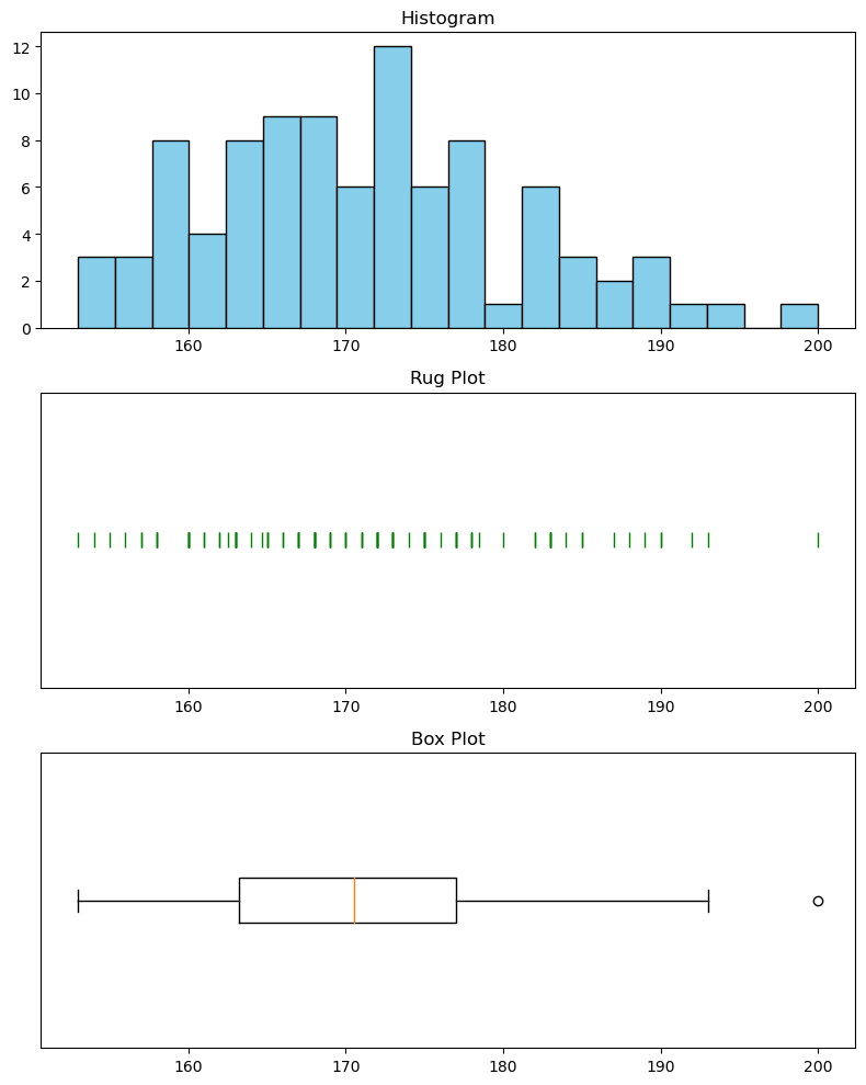
Exercise 5: Try the above code for yourself. Remember to import the necessary libraries and load the gs_intro_survey data.
Exercise 6: Look at each plot. What information do you think each plot shows?
Exercise 7: Experiment with the code and check the documentation to see how much of the code you can understand. Some tips and ideas to try:
- The
subplots()function returns two things:- a figure that contains the whole visualisation, which we store in the
figvariable, and - an array of axes that contains each individual plot, which we store in the
axesvariable
- a figure that contains the whole visualisation, which we store in the
- Try commenting out a line using
#at the beginning so that python ignores the code on that line - Try adjusting the figure size and arranging the plots in three columns instead of three rows.
- Add labels to the (horizontal) x-axis and (vertical) y-axis.
- Experiment with different colours
You can annotate your visualisations to indicate certain values using axvline() and text(). For instance, you can use the following code in the previous example:
axes[0].axvline(184, color='black')
axes[0].text(184, 8,"Leto's height",rotation=90,
             backgroundcolor='white', horizontalalignment='center')
Code for a single figure must all be contained within the same cell code in your notebook. It won’t work across different cells
Exercise 8: Use axvline() and text() to annotate the figure with the averages that we covered last week.
 |
|---|
| Good visualisations help convey your messages.1 |
Measures of variation
Measures of variation are statistical indicators that describe the spread or dispersion of a set of data points. They help us understand how much individual data points deviate from averages, such as the mean or median. Here’s an overview of some common measures of variation:
Range: The range is the simplest measure of variation and is calculated as the difference between the maximum and minimum values in a dataset. It is sensitive to outliers and may not accurately represent the overall variability if extreme values are present.
\[\rm Range = Maximum Value - Minimum Value.\]Variance: The variance measures the mean squared distance of each data point from the mean. A higher variance indicates greater variability, and a lower variance suggests that the data points are closer to the mean.
\[\textrm{Variance}(\sigma^2)= \frac{\sum_{i=1}^n (x_i−m)^2}{n},\]where $n$ is the number of data points, $x_i$ represents each data point, and $m$ is the mean.
Standard Deviation: The standard deviation is the square root of the variance. It is a more interpretable measure of spread, as it is in the same units as the original data. Like variance, standard deviation is sensitive to outliers, but it is widely used due to its ease of interpretation.
\[\textrm{Standard Deviation}(\sigma) = \sqrt{\frac{\sum_{i=1}^{n} (x_i - m)^2}{n}}\]where $x_i$ represents each individual data point, $m$ is the mean and $n$ is the number of data points.
Quartiles: are values that divide a dataset into four equal parts. They help us understand the distribution of the data and identify key points. There are three quartiles in a dataset:
- First Quartile (Q1): This is the value below which 25% of the data falls. In other words, if you order your data from smallest to largest, Q1 is the value at the 25% mark. Also known as the 25th percentile.
- Second Quartile (Q2): This is the median of the dataset. It’s the middle value when the data is sorted. Fifty percent of the data points are below Q2, and fifty percent are above it. Also known as the 50th percentile.
- Third Quartile (Q3): This is the value below which 75% of the data falls. Like Q1, if you order your data, Q3 is the value at the 75% mark. Also known as the 75th percentile.
Interquartile Range (IQR): The interquartile range is a measure of statistical dispersion, or, in simple terms, the range of the middle 50% of the data. It is less sensitive to extreme values than the range, variance, or standard deviation. The IQR is the difference between the third quartile (Q3) and the first quartile (Q1). It represents the spread of the central portion of the data.
\[\rm IQR=Q3−Q1 .\]These measures of variation provide different perspectives on the distribution of data. Researchers and statisticians choose the most appropriate measure based on the characteristics of the dataset and the goals of their analysis.
Exercise 9: Write a function differenceFrom(x, m) that subtracts a value x from m and returns the answer. Set the default value of m to be zero.
Exercise 10: Write a function divideBy(s, n) that divides a number s by another number n and returns the answer.
Exercise 11: Write a function calculateMean(numberList) that calculates the mean of a list of numbers using a for loop. How could you test that your function works correctly?
Exercise 12: Using functions you have written, can you write another function that calculates the variance.
Exercise 13: Think about the definition of variance. The variance aims to capture information about how much we expect values to be different from the mean. Think about the function and/or the formula for variance above. Notice that we compare each data point to the mean. Why is it necessary to square the difference between each data point and the mean? Experiment with the function you wrote to see what happens if you do not square it.
Exercise 14: The standard deviation is considered more easy to interpret because it is in the same units as the data. Use the code below to investigate the standard deviation:
def test_standard_deviation(r, m=10):
    x = np.zeros(10)   # create a dataset of 10 values
    x[:5] = m - r
    x[5:] = m + r
    return x
Look at the output of the function as you change the arguments. How does the mean and standard deviation change as you vary the values of the function arguments?
Hint: you can use numpy.mean(x) and numpy.std(x) to calculate the mean and standard deviation
Exercise 15: Annotate the distribution of heights from earlier to indicate these measures of variation. The statistics functions in numpy will be useful.
Exercise 16: Using everything you’ve learned this week, can you now determine what information the boxplot shows you?
 |
|---|
| And this is why the box plot was invented.2 |
-
Self-Description by xkcd licensed under CC BY-NC 2.5 ↩
-
Boyfriend by xkcd licensed under CC BY-NC 2.5 ↩