Tutorial 8

---

Tutorial Summary:

• Manipulating data in pandas
• Unit of analysis and observation
• Ecological fallacy

---

In this tutorial we will introduce the concepts of unit of analysis and unit of observation and the important issues that can arise in statistical analysis when we do not properly account for the distinction between the two.

Manipulating data in pandas

Pandas is a powerful library for data manipulation and analysis in Python. We’ve already seen how we can use python to read and load .csv data files. Here we’ll cover some essential operations like reading data, selecting and filtering data, creating and deleting columns, and grouping data.

Let’s start by loading some global population data¹. You can download the data here and load it locally from your own machine or load it remotely:

gapminder = pd.read_csv('https://piratepeel.github.io/GlobalStudiesQuantMethodsS1/data/gapminder.csv')

Summarising Data

Once you have your data loaded, you can summarise it using various Pandas DataFrame functions. We’ve already seen the head() function to display the first few rows. Here are a few more summary functions you can try:

# Display the last few rows
print(gapminder.tail())

# Summary statistics
print(gapminder.describe())

# Data types and missing values
print(gapminder.info())

Exercise 1: Try the above functions and observe what they do.

Exercise 2: Notice that the describe() does not summarise all the columns in the data. Which columns does it miss? Why do you think this is?

You can summarise the “missing” columns by using the argument include='object':

gapminder.describe(include = 'object')

Exercise 3: Confirm that the code above summarise the remaining columns. What does each row of the summary tell you?

Selecting and Filtering Data

You can select specific columns and filter rows based on conditions:

# Selecting a single column and save in a new variable
life_expectancy = gapminder['lifeExp']

# Selecting multiple columns
life_exp_and_gdp = gapminder[['lifeExp', 'gdpPercap']]

Exercise 4: Create a scatter plot, in the way that you did last week, of life expectancy and GDP.

You can also filter data using a conditional statement. For example, if you want to only select the data after a given date:

# Filtering rows based on a condition
gapminder_after1984 = gapminder[gapminder['year'] > 1984]

Exercise 5: Can you understand the code above? How does this select rows corresponding to data after 1984? Try just running the conditional statement gapminder['year'] > 1984, what does this produce?

Alternatively you can filter data using the query() function, like this:

gapminder_after1984 = gapminder.query('year > 1984')

Exercise 6: Create a scatter plot of life expectancy and GDP in which the data points corresponding to before and after 1984 are in shown difference colours.

Creating New Columns

You can create new columns based on existing ones (or with new data) simply by defining a new column:

# Create a new column based on existing columns
gapminder['yearsAgo'] = 2023 - gapminder['year']

Grouping and Aggregating Data

Grouping allows you to split the data into groups based on some criteria and then apply a function to each group:

# Group by a column and calculate the mean for each group
yearly_life_exp = gapminder.groupby('year')['lifeExp'].mean()

Exercise 7: Try grouping the data using the code above. What does it do? Try plotting the data. Do you see a pattern?

Note: When you group data, you also need to specify an aggregation function so that pandas knows how to combine all the values in the group. The above example uses mean(), but you can also use other functions such as median() and count() to aggregate values within each group.

Merging DataFrames

With Pandas you can merge two DataFrames based on a common column using the merge() function. This is a powerful technique to allow you to combine data from different sources. For instance:

# Merge two DataFrames df1 and df2 based on a common column
merged_df = pd.merge(df1, df2, on='CommonColumn')

To try this with the gapminder dataset, we will need to load another DataFrame that has information about which continent each country belongs to.

continents = pd.read_csv('https://piratepeel.github.io/GlobalStudiesQuantMethodsS1/data/continents.csv')

We can merge the two DataFrames so that we can analyse the gapminder data by continent. The continents and gapminder DataFrames both have a column that contains country names. However, the columns are named differently. From the merge() function documentation we see that we can specify different column names by replacing the on= argument with left_on= and right_on:

gap_merged = pd.merge(gapminder, continents, left_on='country', right_on='name')

Exercise 8: Try merging the two DataFrames based on country names. Look at the number of rows in each of the original DataFrames and compare with the number of rows in the merged DataFrame. What do you notice. Can you guess why this is?

Note: You can use either the info() or describe() functions mentioned above or the built-in function len() to find the number of rows in a DataFrame.

Hint: Use the unique() function to see the list of country names in each DataFrame:

gapminder['country'].unique()

Exercise 9: There are different ways to merge DataFrames. Create two new merged DataFrames using a left merge and right merge:

gap_merged_left = pd.merge(gapminder, continents, left_on='country', right_on='name', how='left')
gap_merged_right = pd.merge(gapminder, continents, left_on='country', right_on='name', how='right')

Look at the number of rows in these new DataFrames. Does this help you understand what the left and right merges do?

To further investigate what is going on, we can use the isnull() function to identify rows that have missing values. For example, the following code will select the rows in the 'country' column that are missing.

gap_merged[gap_merged['country'].isnull()]

Exercise 10: Investigate the missing values in the 'country' and 'name' columns of the gap_merged_left and gap_merged_right DataFrames. Can you now see the problem that occurs when merging the two DataFrames?

Exercise 11: You can fix the issue by merging based on the ISO country codes. Try this and confirm that you no longer have missing values.

Deleting columns

When you merge DataFrames you may find that you have more columns than you really need for your analysis. For instance, in the previous examples we merged two DataFrames based on the 'country' and 'name' columns that both contain the country name. We might therefore want to delete one of the columns.

gap_merged.drop('name', axis=1)

Exporting Data

Once you have performed these data manipulations, you might want to save the final dataset so that you don’t have to repeat these steps all over again. Save your manipulated data back to a file:

# Save DataFrame to a CSV file
gap_merged.to_csv('merged_gapminder.csv')

This is a basic overview of Pandas operations for data manipulation. As you become more familiar with Pandas, you can explore more advanced functionalities for data cleaning, reshaping, and analysis. The official Pandas documentation is an excellent resource for detailed information and examples.

	Pandas can efficiently handle and manipulate your data2

Unit of analysis and unit of observation

Unit of analysis and unit of observation are concepts used to define what is being studied and measured. While they may sound similar, they refer to distinct aspects of the research process.

Unit of Analysis

The unit of analysis is the level at which the researcher is examining the data. It is the entity or phenomenon that the researcher is interested in making inferences about. This is often a theoretical or conceptual entity that represents the primary focus of the study. It could be a group, an organisation, an individual, or any other defined entity. For example, in a study examining the impact of educational policies on student performance, the unit of analysis might be individual students or classrooms.

Unit of Observation

The unit of observation, on the other hand, is the specific entity or case from which the researcher collects data. It is the unit that is observed or measured in the study. The unit of observation is the concrete, tangible entity from which data is gathered. It could be an individual, a household, a company, etc. Using the same example, if the unit of analysis is individual students, the unit of observation would be specific students selected for data collection.

The difference between unit of observation and analysis

The key distinction lies in the level of abstraction. The unit of analysis is the conceptual entity that the researcher is interested in studying and therefore relates to the scope of the research question. The unit of observation, on the other hand, is the specific, concrete entity from which data is collected and relates more to the practicalities of data collection. In some cases, the unit of analysis and unit of observation may align. For example, when studying individuals in a population, both the unit of analysis and unit of observation could be the same.

In research design, it’s crucial to be clear about both the unit of analysis and the unit of observation to ensure that the research questions are appropriately framed, and the data collection methods are well-suited to answer those questions. In cases that the unit of analysis and the unit of observation are not clear, there can be a risk of making statistical errors known as ecological fallacy.

Important: be careful not to confuse unit of analysis/observation with measurement units such as kilograms, centimetres etc.

Exercise 12: Load the Global Studies Intro Survey that we have been using in the previous tutorials.

1. Group the data by country and display the mean height of global studies students by country.
2. Merge the survey data with the continents DataFrame in such a way that you can group by continent and display the mean heights in each continent. For each case above, what is the unit of observation and what is the unit of analysis?

Ecological fallacy

The ecological fallacy is a logical error that occurs when one makes conclusions about individuals based on group-level data. In other words, it involves mistakenly attributing characteristics or behaviours to individuals based on the characteristics or behaviours of the larger group to which they belong. This fallacy arises when there is a failure to recognise and account for variations within the group.

To understand this concept better, let’s consider an example. Suppose there’s a study that finds a positive correlation between a country’s average income and the average life expectancy of its citizens. If one were to commit the ecological fallacy, they might erroneously conclude that individuals with higher incomes within that country will also have longer life expectancy. However, this conclusion may not hold true when examining individuals within different income levels.

The fallacy arises because averages or correlations at the group level do not necessarily reflect the relationships at the individual level. In the example, while there might be a correlation at the country level, there could be significant variations in life expectancy among individuals with similar incomes.

It’s essential to remember that groups are diverse, and individual experiences within those groups can differ significantly. Relying solely on aggregate data to make inferences about individuals can lead to inaccurate conclusions. Researchers and analysts should exercise caution and consider the potential for individual variations when interpreting data at the group level.

Let’s try some examples in Python to see this fallacy in action.

Exercise 13: Use the code below to summarise the mean monthly income of global studies students by region. Based on this summary who do you think is likely to earn more: a randomly selected student from the Americas or a randomly selected student from Europe?

survey_merged = pd.merge(gs_intro_survey, continents, left_on='Origin', right_on='name', how='left')
survey_merged.groupby('region')['Monthly_Income'].mean()

Exercise 14: The code below simulates 100,000 repetitions of randomly selecting an American and a European and comparing monthly income. What do you notice in the result? Try the same for an American and an Asian student.

# select the data
americas = survey_merged.query('region == "Americas"')['Monthly_Income']
asia = survey_merged.query('region == "Asia"')['Monthly_Income']
europe = survey_merged.query('region == "Europe"')['Monthly_Income']

# Create subplots
fig, axes = plt.subplots(nrows=3, ncols=1, figsize=(8, 4), sharex=True)

# Plot distributions by country
axes[0].hist(americas, color='green', bins=25, range=(0, 3000))
axes[1].hist(asia, color='yellow', bins=25, range=(0, 3000))
axes[2].hist(europe, color='skyblue', bins=25, range=(0, 3000))

axes[0].axvline(np.median(americas), color='black', linestyle=':')
axes[1].axvline(np.median(asia), color='black', linestyle=':')
axes[2].axvline(np.median(europe), color='black', linestyle=':')

axes[0].set_ylabel('Americas', color='green')
axes[1].set_ylabel('Asia', color='yellow')
axes[2].set_ylabel('Europe', color='skyblue')

axes[2].set_xlabel('Monthly Income')

# initialise the counts
equal = 0
america_greater = 0

# number of random simulations
repetitions = 100000

# simulate a lot of random selections
for i in range(repetitions):
    rand_america = np.random.choice(americas)
    rand_europe = np.random.choice(europe)
    if rand_america == rand_europe:
        equal += 1
    elif rand_america > rand_europe:
        america_greater += 1

# print the output
print(f"Equal {equal} time, America greater {america_greater}", 
      f"Europe greater {repetitions - equal - america_greater}")

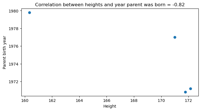
Exercise 15: Run the code below to analyse the relationship between mean heights and the mean year of parent’s birth. Explain whether or not you think this is an ecological fallacy. How could you determine this with the data?

heights = survey_merged.groupby('region')['Height'].mean()
parent_year = survey_merged.groupby('region')['Parent_year'].mean()

correlation = np.corrcoef(heights, parent_year)[0, 1]

fig, axes = plt.subplots(nrows=1, ncols=1, figsize=(8, 4))
axes.scatter(heights, parent_year)
axes.set_xlabel('Height')
axes.set_ylabel('Parent birth year')
axes.set_title(f'Correlation between heights and year parent was born = {correlation:.2f}')

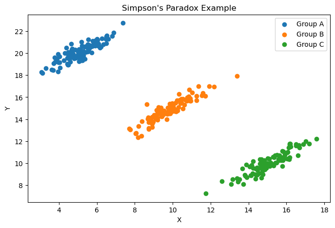
Simpson’s paradox

Simpson’s Paradox is a special case of the ecological fallacy in which combining groups obscures or reverses trends present in individual groups. For instance we might have a positive correlation at the group level, but a negative correlation at the individual level.

For this we can simulate an example using python:

# Set random seed for reproducibility
np.random.seed(42)

# Mean values for the two variables
mean1 = [5, 20]
mean2 = [10, 15]
mean3 = [15, 10]

# Covariance matrix with positive covariance
covariance = [[1, 0.9],
              [0.9, 1]]

# Number of samples in each dataset
num_samples = 100

# Generate three random datasets
data1 = np.random.multivariate_normal(mean1, covariance, size=num_samples)
data2 = np.random.multivariate_normal(mean2, covariance, size=num_samples)
data3 = np.random.multivariate_normal(mean3, covariance, size=num_samples)

# Concatenate the datasets
concatenated_data = np.concatenate([data1, data2, data3])

data = {
    'Group': ['A'] * num_samples + ['B'] * num_samples + ['C'] * num_samples,
    'X': concatenated_data[:, 0],
    'Y': concatenated_data[:, 1]
}

df = pd.DataFrame(data)

# Scatter plot for each group
plt.figure(figsize=(8, 5))
for group in df['Group'].unique():
    group_data = df[df['Group'] == group]
    plt.scatter(group_data['X'], group_data['Y'], label=f'Group {group}')

plt.title("Simpson's Paradox Example")
plt.xlabel("X")
plt.ylabel("Y")
plt.legend()

In summary, the ecological fallacy is a cautionary reminder that relationships observed at one level of analysis, such as a group or population, may not hold true when applied to individuals within that group. It underscores the importance of recognising and addressing the complexities and variations that exist within any given population.

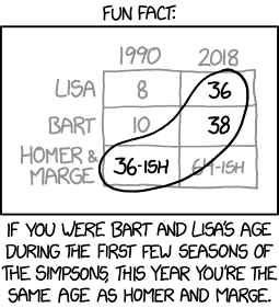
	Be careful not to confuse Simpson’s paradox with The Simpsons paradox.3

1. Data source: https://www.gapminder.org/data/ ↩

2. AI generated image using Canva. ↩

3. The Simpsons by xkcd licensed under CC BY-NC 2.5 ↩