Tutorial Three — Centrality

Reading: Chapter 14 of The Atlas for the Aspiring Network Scientist (2025 edition): Node ranking.

1. In Tutorial 1 you showed that the (i,j) entry of A² counts the number of walks of length 2 between nodes i and j. This exercise picks up that thread and shows that a simple iterative process leads directly to one of the most important centrality measures in network science.

Let A be the adjacency matrix of a simple undirected graph and 1 be the all-ones vector.

(a) In Tutorial 1 you found that A1 gives the degree vector k. What does A²1 compute, and what does its i-th entry represent in terms of the network structure? What about Aⁿ1 for general n?

(b) Consider the following iterative process: start with an arbitrary positive vector x⁽⁰⁾, then repeatedly compute x⁽ᵗ⁺¹⁾ = Ax⁽ᵗ⁾ and normalise so that the vector has unit length. Implement this for a small network of your choice and run it until the vector stops changing. What does the result correspond to? Verify your answer against a library function for eigenvector centrality.

Note on implementation: for large networks, storing the full adjacency matrix as a dense array is memory-intensive and matrix–vector products become slow. Use a sparse matrix representation instead — for example, scipy.sparse in Python — which only stores the non-zero entries. This is good practice whenever implementing any iterative method on networks, and will be required in Exercise 2(c).

(c) The process in (b) is called the power method. Can you explain intuitively why it converges to the leading eigenvector of A? Under what conditions might it fail to converge, or converge to something unexpected? (Hint: think about what happens on a bipartite graph.)

(Optional) (d) The rate of convergence of the power method is governed by the ratio λ₂/λ₁, where λ₁ and λ₂ are the two largest eigenvalues of A — the smaller this ratio, the faster the convergence. Test this numerically by comparing the number of iterations required to converge on (i) a dense ER graph and (ii) a bipartite graph of similar size. Compute the eigenvalues of each using a library function and verify that the convergence behaviour matches the ratio λ₂/λ₁. Why does the bipartite case behave the way it does?

2. Eigenvector centrality has a natural limitation: if a node has no incoming connections, it receives a score of zero regardless of who it connects to. Several centrality measures have been proposed to address this, and they are best understood as a family built on a single idea.

For this exercise, use the OpenFlights network (available at networks.skewed.de) as your primary network, treating it as a directed graph. You may also use other networks of your choice for comparison.

(a) Katz centrality modifies eigenvector centrality by adding a small baseline score β to every node, so that even isolated nodes receive a non-zero score. The Katz centrality vector satisfies:

\[\mathbf{x} = α\mathbf{Ax} + β\mathbf{1}\]

where α < 1/λ₁ is an attenuation factor. Use a library function to compute Katz centrality for the OpenFlights network. How do the top-ranked nodes compare to a simple degree ranking? What does a high Katz score mean in terms of the network?

(b) Alpha centrality generalises Katz by replacing the uniform baseline 1 with an arbitrary exogenous importance vector e, reflecting prior knowledge about node importance:

\[\mathbf{x} = α\mathbf{Ax} + \mathbf{e}\]

Compute alpha centrality for the OpenFlights network using the in-degree vector as the exogenous importance vector e. How do the results differ from Katz centrality, and why? What would be a meaningful choice of e for the airport network specifically?

(c) PageRank can be understood as a normalised variant of Katz centrality adapted for directed graphs, where the importance passed along an edge is divided by the out-degree of the source node (so high-degree nodes do not automatically dominate). Write a function that implements PageRank using the power method. Use a sparse matrix representation for the adjacency matrix (e.g. scipy.sparse) to ensure your implementation scales to networks with thousands of nodes. Check your implementation against a library function.

(d) Using your PageRank implementation, compute scores for the OpenFlights network across a range of teleportation parameter values d ∈ [0.05, 0.95]. How sensitive are the top-ranked airports to the choice of d? At extreme values of d, what does PageRank reduce to, and why?

(Optional) (e) Compare the ranking of airports under degree centrality, Katz centrality, and PageRank. Identify at least two airports whose rankings differ substantially between measures and explain structurally why this is the case. You may find it helpful to look up the airports and their routes directly.

3. Not all centrality questions ask “how important is this node?” Some ask “does this node serve as a bridge or as a destination?” In directed networks, this distinction gives rise to two separate scores for every node — and the algorithm that computes them has a surprising connection to the bipartite network representation you worked with in Tutorial 1.

The HITS algorithm (Hyperlink-Induced Topic Search) assigns each node in a directed network both a hub score and an authority score. A good hub links to many good authorities; a good authority is linked to by many good hubs. The two scores are mutually reinforcing.

Use the Wikispeedia network (available at snap.stanford.edu/data/wikispeedia.html), a directed network of hyperlinks between ~4,600 Wikipedia articles. Nodes are articles; a directed edge from A to B means article A contains a hyperlink to article B. You may also use another directed network of your choice.

(a) Implement the HITS algorithm or use a library function to compute hub and authority scores for the Wikispeedia network. List the top 10 hubs and top 10 authorities. Look up several of these articles on Wikipedia — do the scores make intuitive sense? Describe what characterises a high-hub article and a high-authority article in this context.

(b) Are the highest-scoring hubs also the highest-scoring authorities? Find at least two articles that score high on one measure but low on the other, and explain why in terms of the article’s content and linking structure.

(c) In Tutorial 1, you worked with the bipartite adjacency matrix B of a network. HITS is equivalent to computing eigenvector centrality on two related matrices derived from the directed adjacency matrix A. Hub scores are the leading eigenvector of AAᵀ and authority scores are the leading eigenvector of AᵀA. Verify this numerically for a small directed network. What is the relationship between this and the one-mode projection of a bipartite network from Tutorial 1?

(Optional) (d) The Wikispeedia game challenges players to navigate from one article to a target article using only hyperlinks. Based on your HITS results, which types of articles would make the most useful intermediate stops in a navigation strategy — high-hub articles or high-authority articles? Why? How does this relate to the betweenness centrality of these nodes?

4. Different centrality measures answer different questions about a network, and for any given node they can give very different answers. Learning to read these disagreements is one of the most practically useful skills in network analysis.

The OpenFlights network provides a concrete and interpretable setting for this exercise: airports are nodes, directed flight routes are edges, and you can look up any airport to understand its real-world role.

(a) For the OpenFlights network, compute the following centrality measures for each node: in-degree, out-degree, PageRank, betweenness centrality, and harmonic closeness centrality. Produce a table or visualisation that shows the top 10 nodes under each measure.

(b) The top nodes under degree centrality are likely to be large international hub airports. Identify at least two airports that rank highly on betweenness centrality but are not among the top degree nodes. Look up these airports. What is their geographic or structural role that makes them important bridges in the network?

(c) Now identify at least two airports that rank highly on closeness centrality but not on PageRank. What does high closeness but moderate PageRank indicate about a node’s position in the network?

(d) PageRank and in-degree are correlated but not identical. Find an airport with substantially higher PageRank rank than in-degree rank, and another with substantially lower PageRank rank than in-degree rank. Explain the structural reason for the divergence in each case.

(e) Based on your analysis, which centrality measure would you recommend for each of the following practical questions? Justify your choice.

Which airports, if closed, would most disrupt the global flight network?
Which airports are most reachable from anywhere in the world with the fewest connections?
Which airports are most likely to see early spread of an infectious disease arriving by air?

5. The Medici family’s dominance of Renaissance Florence is one of the most studied examples of how network position translates into real-world power. Now that you have the configuration model from Tutorial 2, you can test the network explanation rigorously.

The Medici family were a powerful political dynasty and banking family in 15th century Florence. The classic network explanation of their power claims that they established themselves as the most central players in the network of prominent Florentine families, occupying the structurally most important position.

Medici network with harmonic centrality

(a) Load the Medici network. Calculate and report the harmonic centrality of each node and rank the families accordingly. Where does the Medici family appear in the ranking? Does the harmonic centrality ranking support the network explanation of their power? Are there any families whose ranking surprises you?

(b) A high centrality ranking is only meaningful if it is higher than what we would expect by chance for a node with that many connections. Using the configuration model from Tutorial 2, generate an ensemble of 1000 random graphs with the same degree sequence as the Medici network. For each node, compute its harmonic centrality across the ensemble and extract the mean and the 25th and 75th percentile bands. Plot these distributions alongside the observed harmonic centrality of each node.

Is the Medici family’s centrality score above what the configuration model predicts for a node with their degree? Which other families, if any, score above or below expectation? What does this tell us about whether the Medici’s structural importance can be explained by their number of connections alone?

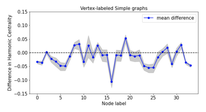
(Optional) (c) The conclusion from (b) may depend on which version of the configuration model you use. Repeat the analysis using the Fosdick et al. MCMC approach to sample from (i) the vertex-labeled simple graph space and (ii) the stub-labeled loopy multigraph space. For each graph space, plot the difference between each node’s observed harmonic centrality and its mean centrality in the ensemble. Do your conclusions about the Medici’s structural advantage change depending on the null model chosen? What does this imply about the importance of being precise when specifying a null model?