Tutorial Six — Exercises

Consensus Dynamics

---

1. The matrix form of the consensus dynamics is:

\[\dot{\mathbf{x}} = -\mathbf{L}\mathbf{x}\]

Show that this is equivalent to the coordinate form:

\[\dot{x}_i = \sum_j A_{ij}(x_j - x_i)\]

(a) Why is it the graph Laplacian L that governs the dynamics, and not the adjacency matrix A? What would the dynamics look like if you replaced L with A?

(b) The update rule is purely local: each node adjusts its state based only on the difference to its immediate neighbours. Yet the system converges to the global mean of the initial conditions. Explain intuitively why this is the case, and state what property of the network is required for this convergence to be guaranteed.

---

2. The second-smallest eigenvalue of the Laplacian, λ₂ (the Fiedler value), controls how quickly the network reaches consensus.

(a) Simulate consensus dynamics on a small synthetic undirected network of your choice (~50 nodes). Assign random initial states to nodes, integrate the dynamics numerically, and verify that the system converges to the mean of the initial conditions. Plot the state of each node as a function of time, and estimate the convergence timescale from your plot. How does this compare to 1/λ₂?

(b) Now run the same simulation on the OpenFlights airport network (available at https://networks.skewed.de/net/openflights). This network is directed. Before simulating, discuss: does consensus dynamics as defined above make sense on a directed network? What modification, if any, would be needed? Run the simulation on the largest weakly connected component and comment on the convergence behaviour.

---

3. In a network with modular structure, consensus dynamics displays timescale separation: nodes within the same community reach approximate consensus long before consensus is achieved across the whole network.

(a) Generate a network using a Stochastic Block Model with 5 equally-sized communities of 60 nodes each (300 nodes total). Choose within-community and between-community connection probabilities such that the block structure is clearly visible in the adjacency matrix. Assign each node a random initial state drawn uniformly from [1, 5].

Reproduce a figure analogous to the figure below: plot the reordered adjacency matrix (panel A) and the evolution of node states on a logarithmic time axis with nodes coloured by community membership (panel B).

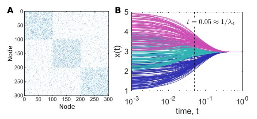
Illustration of consensus dynamics on a structured network. A Adjacency matrix of a network with community structure. B Consensus dynamics on this network with time-scale separation. At the marked time approximate consensus is formed within groups and the a consensus is reached between groups.

(b) The timescale at which local consensus is reached within communities is predicted by t* ≈ $1/\lambda_C$, where $\lambda_C$ is the C-th smallest eigenvalue of the Laplacian and C is the number of communities. Compute the relevant eigenvalues of your network’s Laplacian and verify that they predict the timescale separation visible in your figure.

(c) Vary the ratio of within-community to between-community connection probability. How does this affect: (i) the visibility of block structure in the adjacency matrix, (ii) the timescale separation in the dynamics, and (iii) the spectral gap?

Discussion question: How does the timescale separation observed here relate to the idea of spectral clustering? In what sense is consensus dynamics performing a kind of community detection?