Networks and Simulation — Tutorial Four

Exercises: Community Structure

In these exercises you can choose whichever network software package you prefer. However, for some exercises you will need to use graph tool. In case you cannot install graph tool on your computer, then you can use graph tool in colab.

If you are struggling with the syntax of graph tool, then you use the code from this notebook.

Exercise 1 — Modularity from first principles

Modularity is not an arbitrary score: it follows directly from the null model you built in Tutorial 2. This exercise asks you to derive it and then apply it by hand, so that the formula is something you arrived at rather than something you were given.

(a) In Tutorial 2 you showed that the configuration model predicts an expected number of edges between nodes $i$ and $j$ of $k_i k_j / 2m$. Using this null model expectation, write down a quantity that measures, for a given partition of the nodes into communities, how many more within-community edges there are than the null model predicts. Your expression should sum only over pairs of nodes in the same community and should be normalised so that it lies between $-1$ and $+1$. Compare the formula you arrive at with the modularity formula in the notes.

(b) The network below has 9 nodes and two communities: ${1, 2, 3, 4, 5}$ and ${6, 7, 8, 9}$.

9-node network

Calculate the modularity of this partition. Show your working by first computing the degree of each node and the null model expectation for each within-community pair.

(c) Discussion question. The null model embedded in the modularity formula is the configuration model. What does this tell you about the kind of structure modularity is designed to detect? Are there types of community structure it would not pick up on, or would actively penalise?

Exercise 2 — The resolution limit

Modularity maximisation is the most widely used community detection method, but it has a systematic failure mode that is not obvious from the formula. This exercise demonstrates it on a controlled planted partition network where you know exactly what the communities should be.

(a) Write a function create_ring_of_cliques(k, clique_size) that generates a network consisting of $k$ cliques each of size clique_size, connected in a ring: each clique is linked to the next by a single edge. Use the function to generate a network with $k = 10$ cliques of size 10. Visualise the network and verify that the community structure is visually clear.

(b) Apply modularity maximisation to the network from (a) using the Louvain algorithm (e.g., via the python-louvain package or igraph’s community detection). How many communities does it recover? Do the recovered communities correspond to the planted cliques?

# Example using igraph
import igraph as ig
import leidenalg  # alternative: community_multilevel in igraph

g = ig.Graph.Famous("Petersen")  # replace with your ring-of-cliques graph
partition = g.community_multilevel()
print(len(partition))  # number of communities found

(c) Now generate networks with $k \in {2, 3, 5, 10, 20, 50, 100, 150}$ cliques of size 10. For each, apply modularity maximisation and record the number of communities returned. Plot the number of detected communities against $k$. At approximately what value of $k$ does modularity begin to fail?

(d) Discussion question. The resolution limit of modularity is approximately $\sqrt{m}$, where $m$ is the total number of edges. Check whether this prediction is consistent with where your plot begins to diverge. What does this tell you about using modularity on large networks where you expect many small communities? Would increasing the clique size help or hurt?

Exercise 3 — Modularity, null hypothesis testing, and the SBM

Detecting communities and confirming community structure are not the same thing. This exercise works through three networks — each designed to illuminate a different aspect of what methods actually test — and asks you to think carefully about what each result means.

(a) Network One: clear planted partition

The following code generates a planted partition network with 10 communities of 100 nodes each, with strong within-community connectivity and weak between-community connectivity.

import graph_tool.all as gt
from graph_tool import topology, inference, generation
import numpy as np

def prob(a, b):
    if a == b:
        return 0.9
    else:
        return 0.01

g1, bm = generation.random_graph(
    1000,
    lambda: np.random.poisson(10),
    directed=False,
    model="blockmodel",
    block_membership=lambda: np.random.randint(10),
    edge_probs=prob
)

Visualise the network using gt.arf_layout and colour nodes by their planted community membership. Apply modularity maximisation and the SBM to detect communities. For each method, report the number of communities found and compare the recovered partition to the planted partition.

Discussion question. Both methods should perform well here. Why is this case not very informative about which method is better?

(b) Network Two: no community structure

The following code generates an Erdős–Rényi random graph with the same mean degree as Network One — no planted structure.

g2 = generation.random_graph(1000, lambda: np.random.poisson(10), directed=False)

Apply modularity maximisation to g2. What partition does it return, and what is the maximised modularity value?

To evaluate whether this result is meaningful, perform a null hypothesis test. Generate 1000 rewired versions of g2 using generation.random_rewire (this preserves the degree sequence, as in Tutorial 2), apply modularity maximisation to each, and record the maximised modularity values. Plot the null distribution alongside the value you obtained for g2. Compute the p-value.

Note: comparing observed modularity against a rewired null is a natural extension of the null model logic from Tutorial 2, but it is not the most common practice in the literature — it is computationally expensive and requires running modularity maximisation many times. The references for why random graphs have non-zero expected modularity are Guimerà et al. (2004) and McDiarmid and Skerman (2013).

Now apply the SBM to g2. What does it return?

Discussion question. What do these two results together tell you? Even if the null hypothesis test returns a significant p-value, what does that confirm, and what does it not confirm? What is the SBM doing differently from the null hypothesis test?

(c) Network Three: embedded structure

Network Three is an ER random graph with a near-complete clique embedded in a subset of nodes.

g3 = generation.random_graph(1000, lambda: np.random.poisson(10), directed=False)

clique_size = 25
for i in range(clique_size):
    for j in range(i + 1, clique_size):
        g3.add_edge(i, j, add_missing=False)

Apply modularity maximisation to g3. How many communities does it find? Perform the null hypothesis test again: does the test reject the null hypothesis of no structure?

Now apply the SBM. What does it return?

Discussion question. This is the key case. Modularity finds multiple communities and the null hypothesis test is significant. Does this confirm that the network has multiple communities? What is the SBM actually detecting, and why does it give a more direct answer to the structural question you care about? What does it mean that the null hypothesis test is significant but the SBM returns a simpler model?

(d) (Optional) Network Four: metadata and community structure

The political books network records co-purchasing links between books about US politics, with each book labelled liberal, conservative, or centrist.

g_books = gt.collection.data['polbooks']

Apply the SBM to this network. Compare the recovered partition to the known metadata labels stored as a node property.

Discussion question. If the SBM communities do not perfectly recover the political labels, what does that tell you? Is the SBM wrong, or is the metadata capturing something different from community structure in this network? What would you need to know to distinguish between these explanations? This question does not have a single correct answer.

Exercise 4 — Degree-correction and model selection

The standard SBM assumes that within each community nodes have similar expected degrees — the community is internally an ER graph. The degree-corrected SBM relaxes this, treating each block as a configuration model graph instead. This exercise asks you to compare the two models and interpret what the comparison tells you about the data.

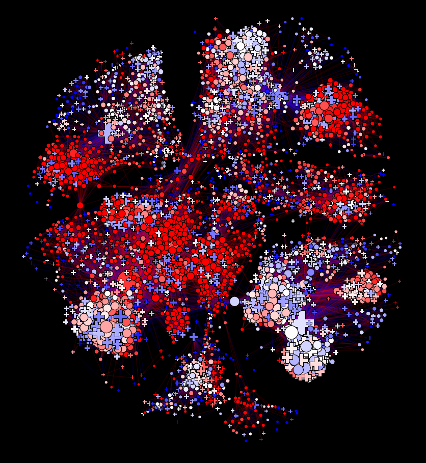
The political blogs network connects blogs about US politics with known left/right labels and a highly heterogeneous degree distribution.

g_polblogs = gt.collection.data['polblogs']
g_polblogs = topology.extract_largest_component(g_polblogs, prune=True)
gt.graph_draw(g_polblogs,
              vertex_fill_color=g_polblogs.vp['value'],
              pos=g_polblogs.vp['pos'])

(a) Fit the standard SBM (deg_corr=False) to the polblogs network, constraining the search to two communities (B_max=2). Report the entropy (description length) and visualise the resulting partition.

(b) Fit the degree-corrected SBM (deg_corr=True) with the same constraint. Report the entropy and visualise the resulting partition.

(c) Compare the description lengths from (a) and (b). The model with the lower entropy provides the more parsimonious description. Which model is preferred? Visualise the within-community degree distributions for both models and describe what you see.

(d) Discussion question. Why would the DC-SBM be preferred for a network with a heterogeneous degree distribution? Connect your answer to what the configuration model preserves that the ER model does not (Tutorial 2, Exercise 4). Under what circumstances might the simpler SBM still be the better choice?

(Optional) Remove the B_max=2 constraint and refit both models. Does the preferred number of communities change? What does this tell you about how degree heterogeneity and community structure interact in the inferred model?

Exercise 5 (Optional — choose one of Exercises 5 or 6) — Detectability and the eigenvalue spectrum

There is a fundamental limit to community detection: below a certain signal-to-noise threshold, no algorithm can recover a planted partition better than chance. This is not a limitation of any particular method — it is an information-theoretic property of the network. This exercise makes that limit visible through the eigenvalue spectrum of the adjacency matrix.

(a) Generate three planted partition networks, each with $n = 1000$ nodes and $k = 2$ equally sized communities, at three different signal-to-noise regimes:

Easy: $p_\text{in} = 0.05$, $p_\text{out} = 0.005$
Marginal: $p_\text{in} = 0.02$, $p_\text{out} = 0.015$
Impossible: $p_\text{in} = p_\text{out} = 0.015$ (i.e., an ER graph)

For each network, compute the eigenvalue spectrum of the adjacency matrix and plot the three spectra side by side.

(b) In each spectrum, identify the dense bulk of eigenvalues and any eigenvalues that appear separated from it. How many outlier eigenvalues are present in each case? How does this relate to the number of planted communities?

(c) Apply the SBM to each of the three networks. Is the number of communities returned consistent with the number of outlier eigenvalues you observed?

(d) Discussion question. The detectability threshold in the planted partition model occurs approximately when $(p_\text{in} - p_\text{out}) / \sqrt{\langle k \rangle}$ falls below 1. Compute this ratio for your three networks. Does the eigenvalue spectrum reflect this threshold? What does this imply for practitioners: if you run community detection on a real network and find no communities, what might that mean?

Exercise 6 (Optional — choose one of Exercises 5 or 6) — Community structure in the airport network

You analysed the OpenFlights airport network in Tutorial 3. Here you apply community detection to the same network and ask how the communities relate to the centrality results you already computed.

(a) Load the OpenFlights airport network (undirected, largest connected component) using the same source as in Tutorial 3. Apply the SBM and report the number of communities found. Visualise the network with nodes coloured by community membership.

(b) Do the recovered communities correspond to geographic regions? Airports in the OpenFlights dataset have latitude and longitude attributes. Map the communities geographically and describe what you observe.

(c) In Tutorial 3 you computed betweenness centrality for this network. Compare the most central airports (by betweenness) to the community structure: do high-betweenness airports tend to sit at community boundaries or within communities? Why would you expect this, based on what betweenness centrality measures?

(d) Discussion question. Geographic region is a form of metadata. Do the SBM communities correspond to geography, or do they capture a different aspect of the network’s structure? What factors other than geography might explain the communities you observe? Does any mismatch between geographic regions and SBM communities tell you something about how the global air transport network is organised?